模型的白盒测试和黑盒测试
黑盒测试-模型结构的推测与补全
首先在仅给模型文件的情况下,我们需要通过其他方式,将常见的一些模型进行推测出来。这边通过两道例题演示相关方法。
我们需要先知道如何去读取Pth模型文件,探求模型的参数结构。
-
1
2
3
4
5
| import torch
#自行选用cpu或者gpu
pt = torch.load("./model.pth", map_location="cpu")
for i in pt:
print(i,pt[i].shape)
|
2.可视化的开源工具
https://github.com/lutzroeder/netron
这边我们选用两道题目作为实例,一个经典的手写LeNet模型,选自2023香山杯
,一个是L3HCTF2021-DeepDarkFantasy,使用动态调试的方法逆向
2024香山杯-LeNet
题目所给出的文件有以下:
- label.json
- MyLeNet.pt
- flag(使用npy格式存储)
先读取模型参数推测
 1
 2
 3
 4
 5
 6
 7
 8
 9
10
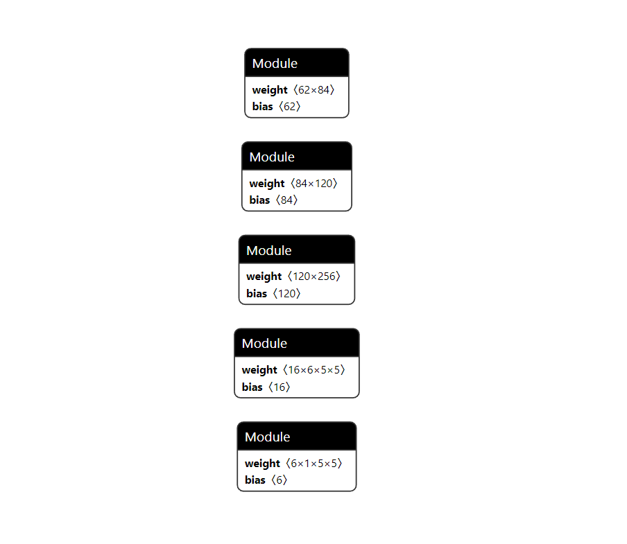
| conv1.weight torch.Size([6, 1, 5, 5])
conv1.bias torch.Size([6])
conv2.weight torch.Size([16, 6, 5, 5])
conv2.bias torch.Size([16])
fc1.weight torch.Size([120, 256])
fc1.bias torch.Size([120])
fc2.weight torch.Size([84, 120])
fc2.bias torch.Size([84])
fc3.weight torch.Size([62, 84])
fc3.bias torch.Size([62])
|
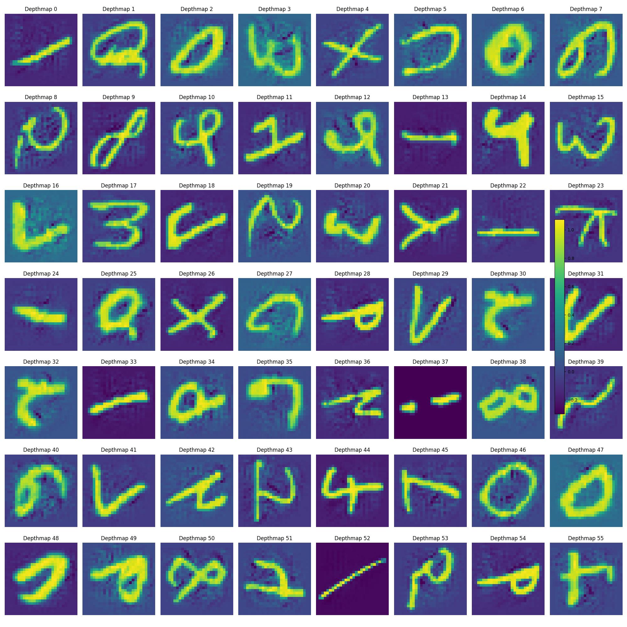
并且呢,我们再将npy进行可视化一下,明显是手写数字+字母
 1
 2
 3
 4
 5
 6
 7
 8
 9
10
11
12
13
14
15
16
17
18
| import numpy as np
import matplotlib.pyplot as plt
rows = 7 # 7行
cols = 8 # 8列
fig, axes = plt.subplots(rows, cols, figsize=(20, 20))
for i in range(56):
depthmap = np.load(f'./flag/{i}.npy') # 使用numpy载入npy文件
ax = axes[i // cols, i % cols] # 确定当前子图位置
im = ax.imshow(depthmap, cmap='viridis')
ax.set_title(f' {i}') #
ax.axis('off')
fig.colorbar(im, ax=axes, orientation='vertical', fraction=0.02, pad=0.04)
plt.tight_layout()
plt.savefig('./pic/all.jpg')
plt.show()
|
这边是给出了相关两个方式都可以查看出存在两个卷积层和三个全连接层,并且给出了其中的基本参数,我们需要去对比一下跟标准的LeNet模型有什么区别,或者说还缺少什么。
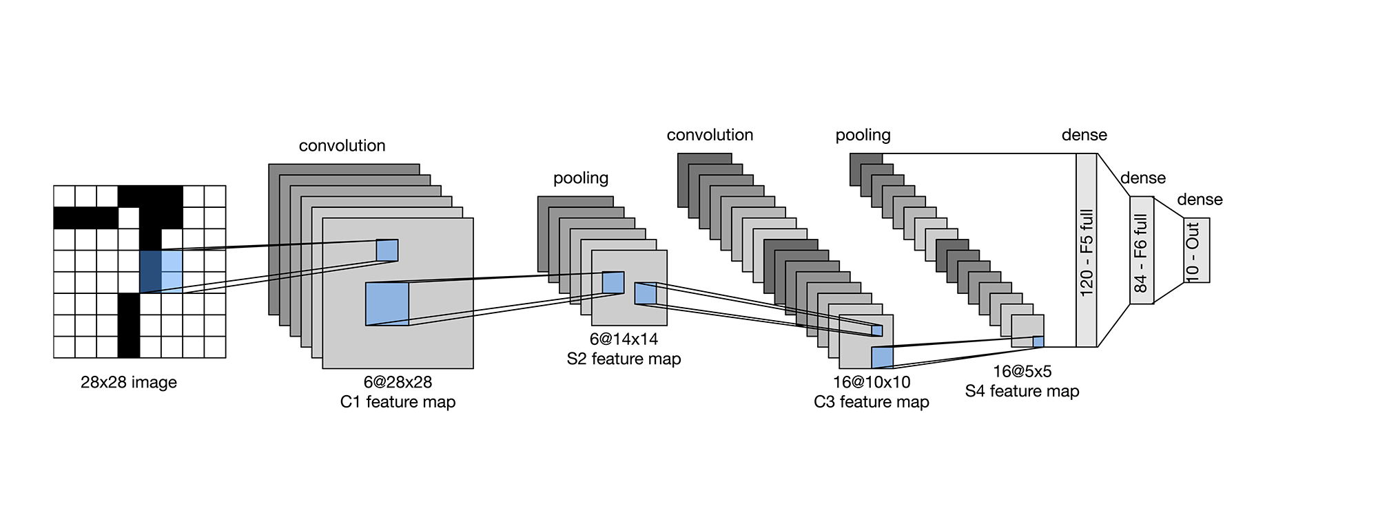
我们发现在经典的LeNet模型,可以发现每次卷积后会进行池化,此处池化我们进行简单化考虑,采用最大池化,因此重点是考虑关于激活函数的问题。
(PS:实际在LeNet网络中,通常使用Sigmoid或Tanh激活函数在全连接层中,而在卷积层中可能使用Sigmoid、Tanh、ReLU等)
我们这里通过实际对模型的逆向查看,发现存在的仅有ReLU函数和Sigmoid函数(PS:如何逆向,010硬看,能搜索到)
需要使用到激活函数的一共有四个位置,卷积层或者全连接层的连接处,上面说明了一共两个卷积层,三个全连接层,因此需要使用到的是四个激活函数,卷积层需要搭配池化。
因此最终的可能性一共在 为16种情况。
此外,还要注意在识别后需要对标签进行映射得到最终的FLAG
 1
 2
 3
 4
 5
 6
 7
 8
 9
10
11
12
13
14
15
16
17
18
19
20
21
22
23
24
25
26
27
28
29
30
31
32
33
34
35
36
37
38
39
40
41
42
43
44
45
46
47
48
49
50
51
52
| import torch
import torch.nn as nn
import json
import numpy as np
pt = torch.load("./MyLeNet.pt", map_location="cpu")
class LeNet(nn.Module):
def __init__(self):
super(LeNet, self).__init__()
self.conv1 = nn.Conv2d(in_channels=1, out_channels=6, kernel_size=5, stride=1)
self.maxpool1 = nn.MaxPool2d(kernel_size=2, stride=2)
self.conv2 = nn.Conv2d(in_channels=6, out_channels=16, kernel_size=5, stride=1)
self.maxpool2 = nn.MaxPool2d(kernel_size=2, stride=2)
self.fc1 = nn.Linear(256, 120)
self.fc2 = nn.Linear(120, 84)
self.fc3 = nn.Linear(84, 62)
def forward(self, x):
x = self.conv1(x)
x = self.maxpool1(x)
x = nn.Sigmoid()(x)
x = self.conv2(x)
x = self.maxpool2(x)
x = nn.ReLU()(x)
x = torch.flatten(x, start_dim=1)
x = self.fc1(x)
x = nn.Sigmoid()(x)
x = self.fc2(x)
x = nn.ReLU()(x)
x = self.fc3(x)
return x
# 创建LeNet实例
lenet_model = LeNet()
lenet_model.load_state_dict(pt)
with open('./label.json', 'r') as json_file:
label_mapping = json.load(json_file)
reverse_label_mapping = {v: k for k, v in label_mapping.items()}
# 获取所有标签
chars = list(reverse_label_mapping.values())
predicted_chars = [] # 用于保存所有的预测字符
for i in range(56): # 从0到56
npy_file_path = f"./flag/{i}.npy"
npy_data = np.load(npy_file_path).reshape((1, 1, 28, 28))
torch_input = torch.tensor(npy_data).float() # 转换为PyTorch张量
# 使用LeNet模型进行推理
output = lenet_model(torch_input)
predicted_index = torch.argmax(output, dim=1).item()
predicted_char = chars[predicted_index]
print(f"Prediction for {npy_file_path}: {predicted_char}")
predicted_chars.append(predicted_char)
result_string = ''.join(predicted_chars)
print("Concatenated Result:", result_string)
|
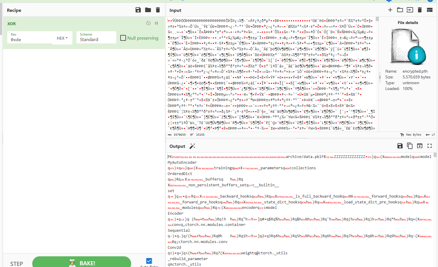
2021L3HCTF-DeepDarkFantasy
直接打开encrypted.pth
先进行异或,KEY为0xde
使用调试的方法逐步补全模型
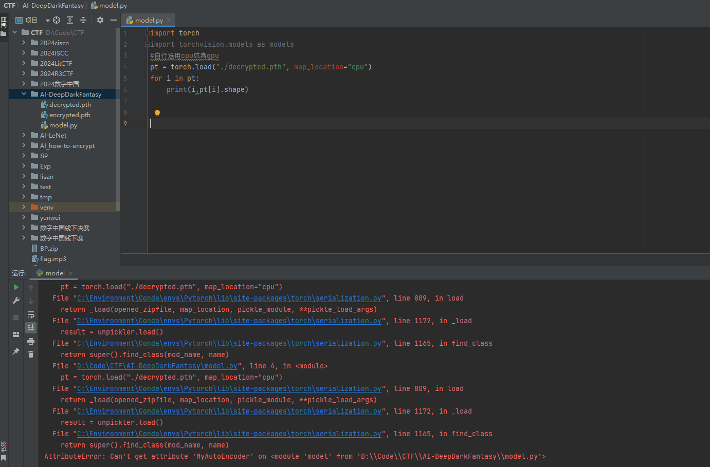
白盒测试-模型的逆向工程
纯粹的模型逆向,先来分析一下初始代码
 1
 2
 3
 4
 5
 6
 7
 8
 9
10
11
12
13
14
15
16
17
18
19
20
21
22
23
24
25
26
27
28
29
| import torch
import torch.nn as nn
flag=''
flag_list=[]
for i in flag:
flag_list.append(ord(i))
input=torch.tensor(flag_list, dtype=torch.float32)
n=len(input)
class Net(nn.Module):
def __init__(self):
super(Net, self).__init__()
self.linear = nn.Linear(n, n*n)
self.conv=nn.Conv2d(1, 1, (2, 2), stride=1,padding=1)
def forward(self, x):
x = self.linear(x)
x = x.view(1, 1, n, n)
x=self.conv(x)
return x
mynet=Net()
mynet.load_state_dict(torch.load('model.pth'))
output=mynet(input)
with open('ciphertext.txt', 'w') as f:
for tensor in output:
for channel in tensor:
for row in channel:
f.write(' '.join(map(str, row.tolist())))
f.write('\n')
|
将字符串转换为ascii码后化为向量,利用一个神经网络,主要是包含全连接层和卷积层,将向量输出。
关于这个网络,我们打印出模型数据,详细过程如下:
1
2
3
4
5
6
7
8
9
| import torch
pt = torch.load("./model.pth", map_location="cpu")
for i in pt:
print(i,pt[i].shape)
#linear.weight torch.Size([2209, 47])
#linear.bias torch.Size([2209])
#conv.weight torch.Size([1, 1, 2, 2])
#conv.bias torch.Size([1])
|
- 输入处理:
- 输入是一个长度为
47 的向量。 - 通过线性层变换为一个长度为
2209 的向量。 - 重塑张量:
- 将长度为
2209 的向量重塑为 [1, 1, 47, 47] 的四维张量。 - 卷积操作:
- 卷积层应用一个
2x2 的卷积核,保持输出形状为 [1, 1, 47, 47]。
同时,我们看到这里存在有n的未知参数,上述我们已经通过读取模型方式获取到n的初始值为47
因此本题的重点也就是放在卷积层和全连接层的逆向操作
卷积层的逆向取决于nn.Conv2d的操作,核心思想是将外围补零后进行逆向操作
Other
其他的就是一些对抗生成模型,算是一个非常热门的考点,或者一些基于论文的AI模型安全问题,目前来说,这个方向资料相对比较少,也没有一个成熟的体系化建设,更多的需要继续去发掘。